My plan was to use neuroevolution to learn how to play a simple video game, but sadly I ran out of time. Fast forward to the end of the year and we had the opportunity to run a week-long experiment of innovation at Black Pepper. Four of us decided to try mob programming, and continuing where I left off, see if we could evolve a video games master.
We first needed to decide on a game for our bot to play. The choice depended on whether to use an emulator to play a real game, or whether to write a simple game from scratch. We settled on the latter for two reasons: it would allow us to modify the game dynamics and observe how it affected the AI; and we wouldn’t have to learn how to programmatically control an emulator and obtain game state for our bot to base decisions upon.
With this in mind we opted for the video game classic Pong. My original neuroevolution code was in Java so we wrote a simple Pong clone in Swing, keeping the game graphics lo-res and omitting match score for simplicity. At this point both players had manual controls so we could enjoy play testing the game.
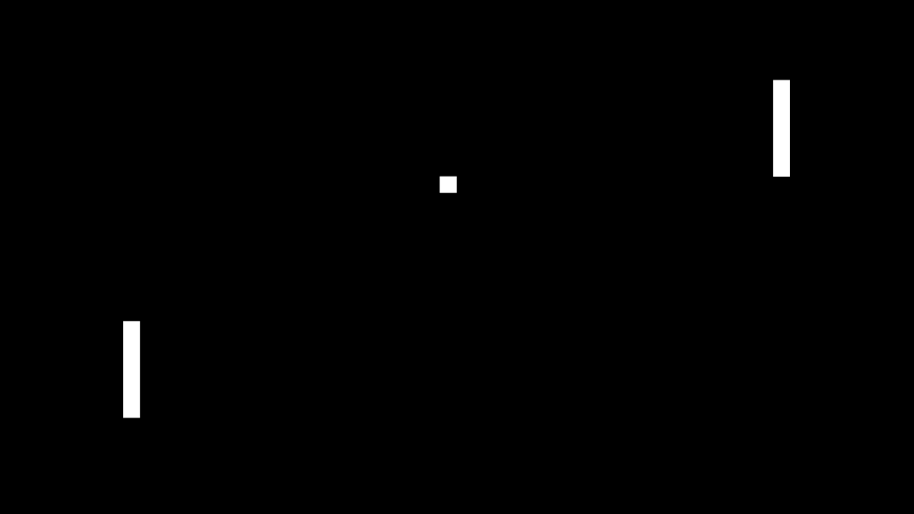
Humans playing Pong
Now that we had the basic infrastructure in place the next step was to start wiring up the neuroevolution library to the game. If this blog post were a film then this part would be the montage. Alas, we were deprived of such luxury and duly proceeded to break this nebulous task into manageable chunks.
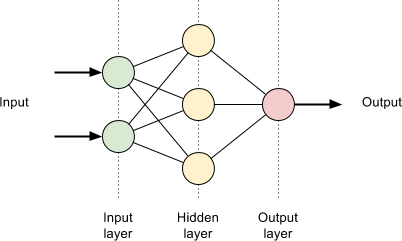
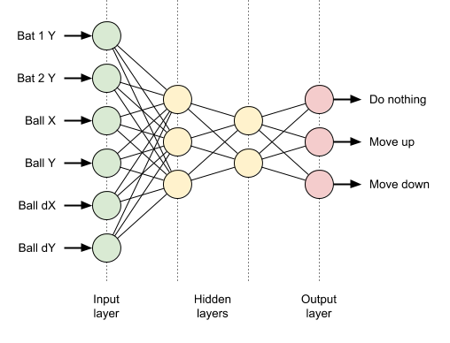
We decided that the simplest form of integration would be to take a genome, which in neuroevolution is a neural network, feed it the game state, and then use the output to move the player. This required us to tie down exactly what the inputs and outputs of the network would be.
If we were playing a more complicated game than Pong then a reasonable approach for the inputs would be to map each node to a lo-res pixel. This felt like an overkill for Pong though, so we settled on six input nodes mapped to the following game state: the bats’ positions, the ball’s coordinates, and the ball’s velocities.
The outputs seemed more obvious. In Pong the player can either move the bat up or down. Less apparent is that they can also elect to do nothing, which we included as an option to encourage the bot to be less hyperactive. Thus we modelled the outputs with three nodes, one for each option, where the strongest signal wins.
Now that we could supply the inputs and act upon the outputs, the remaining task was to feed the data through the network to connect them up. Intuitively one envisages the data propagating forward through the network, indeed this is how classic matrix-based forward propagation is implemented, but with an irregular shaped network it was actually simpler to pull data from the output nodes. This was predominantly due to recursion providing a more concise solution to evaluating a variable number of different sized hidden layers.
We now had enough pieces of the puzzle to assemble our first bot. To validate this we created a random neural network, and with a fortuitous strike of lightning, unleashed it onto a game of Pong and declared it’s alive!
A random genome twitching
One genome playing Pong was a good start, but to harness genetic algorithms we needed entire populations to play Pong. Alongside this we also required a method to identify strong contenders by assigning a fitness score to each one.
We expanded our single genome to an initial population of random genomes and played them out sequentially. To measure their success we simply counted the number of frames that they were alive before the ball went out; the reasoning being that the more often they returned the ball, the better the bot was at playing Pong.
Playing out a population in sequence
As entertaining as it was to watch each match in realtime, we needed a faster approach before we considered evolving multiple generations. To achieve this we introduced a headless mode to the game that bypassed plotting graphics and just updated the in-memory game state. As no-one was watching these games we could also increase the frame rate. Together these changes reduced the time taken to evaluate a population down to fractions of a second.
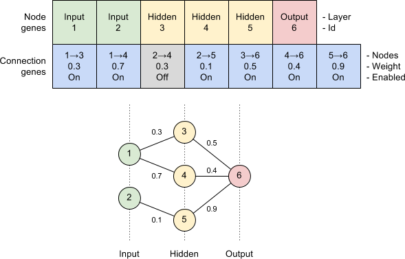
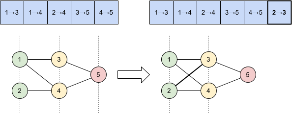
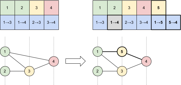
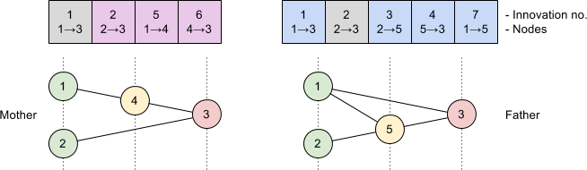
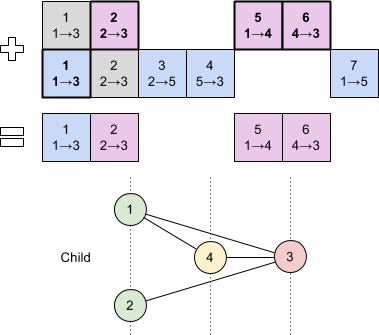
All that now remained between us and evolving King Pong was to implement the standard genetic algorithm loop. I covered much of this in my previous post so I’ll skim over it here. We used roulette wheel selection to choose bots to breed and performed crossover and mutation as specified by NEAT. Once this grunt work was done we could evolve the next generation from the initial population, repeating the process until we were satisfied with our bot’s Pong playing skills.
To help visualise the learning process we selected the fittest bot from each generation and played them sequentially:
Playing out the fittest from each generation
Our bot was now evolving just enough to return the ball, but not a neuron more. Without another player the ball typically went out and it was game, set and match. In order to train the bot further we needed the other player to return the ball for another shot.
This is a perfect situation for coevolution. The idea is that we would evolve another bot that controls the second player alongside evolving the first. Their populations would be distinct, so no cross-breeding, resulting in their behaviour evolving much like an arms race: each time one player learns a new trick, so must the other player learn how to combat it.
As exciting as this would have been to try, we felt that this would complicate matters before we could confidently evolve a single player. Deferring that idea for now we simply replaced the other player with a solid wall. As every bored kid knows, a wall always returns a ball.
A perfect player against a wall
This small change resulted in our bot becoming more sentient than we had catered for. It soon learnt how to play the perfect game and our simulation never ended. To prevent this we introduced a timeout that would terminate the game after so many frames.
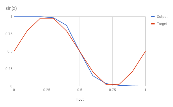
Now that we were getting some genuinely interesting behaviour we wondered what exactly we had evolved. To help visualise the bot we added support to output the neural network as Graphviz. Here is the genome playing the game above:
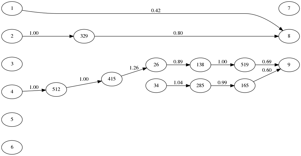
Matching the inputs and outputs to those described earlier, we can see that the bats’ positions are linked to moving up and the ball’s y-coordinate is linked to moving down. As the strongest signal wins, this network represents a seesaw between the ball position causing the bat to move in one direction, and the bat’s new position then causing it to move in the other direction. Note that there is some evolutionary deadwood here that has no net effect but was pivotal to obtaining this structure.
At this point we thought it would be fun to tweak the game dynamics and see how it affected evolution. After reading about the history of Pong for some light relief, we learnt how the original game had a bug whereby the bat was unable reach the extremities of the screen. Allan, the creator of Pong, decided to rebrand this bug a feature so that even a perfect player had a chance of losing. After adding this to the game we noted that it actually slowed down training; presumably due to even perfect players losing and consequently their good genes being deselected.
It was becoming obvious that our simple ball collision mechanics made for rather predictable bots. In the original game of Pong, the contact point of the ball against the bat determines the ricochet angle. Implementing this would require the ball to have fractional velocity, and hence moving our game from lo-res to hi-res graphics. Unfortunately we ran out of time doing this as everything’s more complicated in an unquantised world.
One final aspect of neuroevolution that we didn’t touch on during this experiment was speciation. This protects innovation against ruthlessly pursuing survival of the fittest. We have since had a chance to revisit this and added preliminary support for species which resulted in much more sophisticated behaviour.
A bot evolved with speciation
You can find our resultant neuroevolution library on GitHub, along with the Pong demo. Perhaps next time we’ll finish hi-res graphics, speciation, and coevolution. Until then, let us know if you have any success integrating it with other games and any feedback is always welcome.
]]>I was inspired by the above video shared by a colleague of a program learning how to play Super Mario World. Without human intervention it goes from mashing random buttons to mastering the level. The technique behind this seemingly magical feat is known as neuroevolution – a combination of genetic algorithms and neural networks. It was this that I set out to understand.
Genetic algorithms take their inspiration from biology’s natural selection. They work by decomposing solutions to a problem into genes and chromosomes, scoring them against a fitness function, and then breeding the best together to evolve a more optimal set of solutions. To better understand this I decided to write a program that evolves the string HELLO WORLD
from random characters.
In this simplistic case genes are characters and chromosomes are strings. We start the process with a population of random strings and evolve them until we produce the chosen one. Evolving the population involves repeatedly selecting two parents to produce offspring for the next generation in a process known as crossover. There are a number of techniques available for selection and crossover; I chose roulette wheel selection and single point crossover with random mutation respectively. The fitness function I used for selection simply summed the number of correct characters that were in their correct place.
Take a look at GeneticAlgorithmDemo to see how this looks in code. Running this outputs the fittest individual in each generation:
# 1 QEOCKXWOEJS
# 2 HFLKVSWCRGZ
# 3 HFLKVSWOTLL
# 4 HZILFNWOGLD
# 5 HZILFNWOGLD
# 6 HELBS WCRQD
# 7 HVLNO WOEJD
# 8 HETLFNWOGLD
# 9 HELNONWOGLD
# 10 HELLO WOEJD
# 11 HZLLO WOGLD
# 12 HEL O WOWQD
# 13 HELLO WOEGS
# 14 HELLO WOJJD
# 15 HEL O WOWLD
# 16 HELLO WORGD
# 17 HELLO WORGD
# 18 HELLO WORGD
# 19 HELLO WOELD
# 20 HELLO WORLD
Found HELLO WORLD in 20 generations!
In this run, starting from random characters we arrived at our desired string in twenty generations.
I later learnt that Richard Dawkins proposed a similar thought experiment under the guise of the Weasel program. As an aside, it’s worth noting that this use of natural selection can be misleading as it presupposes a goal, much like intelligent design. This is only because our fitness function is overly precise. Perhaps a better example would have been to evolve a string that consists of two English words, where HELLO WORLD
is only one possible solution.
With genetic algorithms under my belt, the next technique I needed to understand was neural networks. Even from a technical perspective, neural networks are enigmatic beasts. They attempt to solve problems that are traditionally hard to program algorithmically by mimicking our limited understanding of the human brain.
A simple neural network consists of three layers of neurons connected by synapses. The first layer receives the input, transforms it through weights on its synapses to a hidden layer, which in turn transforms it to the final layer for output. This flow of data through the network is known as forward propagation. The input can be anything that represents the problem at hand, for example pixel values in image recognition, and the output represents the computed answer, like whether it’s a hotdog or not.
The magic of neural networks lies in fine-tuning the transformation of the input data as it’s pushed through the layers. This technique is known as back propagation and it is key to how neural networks appear to learn. The idea starts by feeding an input through the network and comparing the output with the expected result. The difference is passed through a cost function and then used to adjust the synapses a layer at a time from the output back to the input. Repeating this process with many different inputs results in the network starting to reflect the desired behaviour. The theory behind this is rather maths heavy; I’d recommend watching Neural Networks Demystified for an in-depth explanation.
To test my understanding I set about a writing a neural network that could learn the sine function. This would be a network that consisted of a single input neuron for x, three hidden neurons, and an output neuron that gave an approximation of sin(x). Both inputs and outputs are normalised to be between zero and one for simplicity. I trained it with a 100,000 iterations of only three inputs and then asked it to compute sin(x) for ten different inputs. Running the resultant code NeuralNetworkDemo shows how the network improves during training:
Learning...
Iteration | Cost
# 0 | 0.090582
# 10000 | 0.000709
# 20000 | 0.000343
# 30000 | 0.000225
# 40000 | 0.000167
# 50000 | 0.000132
# 60000 | 0.000109
# 70000 | 0.000093
# 80000 | 0.000081
# 90000 | 0.000072
# 100000 | 0.000065
Here we see that the value of the cost function, which quantifies the difference between the actual and expected outputs, diminishes every iteration. Once training has taken place we can then feed our ten different inputs into the network to compute the sine function:
------------ Paste into spreadsheet ------------
Input Output Target
0.0 0.9999873069902044 0.5
0.1 0.9998488493115462 0.7938926261462366
0.2 0.9983090528423926 0.9755282581475768
0.3 0.9833851545556364 0.9755282581475768
0.4 0.8745132768612006 0.7938926261462367
0.5 0.4985759605781311 0.5000000000000001
0.6 0.14886659877620845 0.2061073738537635
0.7 0.0367033795608045 0.024471741852423234
0.8 0.010115911146936 0.02447174185242318
0.9 0.0033188579267310124 0.20610737385376332
1.0 0.001293026219153508 0.4999999999999999
------------------------------------------------
As the output suggests, we can plot this as a graph:
Given the limited set of training data we can see that the network has approximated the sine function quite well. The training data points 0.25, 0.5 and 0.75 are spot on, but the obvious discrepancies are at the extremities. It’s fair to say that these points cannot be inferred from the training data, but we may also be hitting a limitation of the number of neurons in the network, or the fact that the neurons do not support a bias.
Now that I had a basic understanding of genetic algorithms and neural networks I was finally ready to combine the two and delve into neuroevolution. What differentiates this technique from classic neural networks is that it does not require supervision to learn, rather it employs genetic algorithms to evolve the shape and values of the network.
In some respects this means that neuroevolution is simpler than regular neural networks since it doesn’t require backpropagation, which is often the most complex part of any implementation. Instead, the typical genetic algorithmic cycle of measuring fitness, genetic crossover and mutation iteratively trains a population of networks.
This conceptually simple idea quickly poses some difficult questions. How best to encode a neural network into genes and chromosomes? How can we mutate and combine networks to produce offspring? How can we allow beneficial traits in networks to evolve? The approach used by the Super Mario World demo is called NEAT, or NeuroEvolution of Augmenting Topologies.
NEAT encodes neurons and synapses as node and connection genes respectively. A node gene simply states which layer it lives in, whereas a connection gene specifies which nodes it connects, its weight and an enabled flag. Additionally, every time a connection is created a global innovation number is incremented and assigned to the gene. We will see later how this innovation number is used to perform crossover.
Mutation of the network can occur in several ways: connection weights are perturbed; unconnected nodes are connected; and connections are split by introducing new nodes. These basic transformations allow an arbitrarily complex neural network to evolve over time.
To illustrate, a connection gene mutation simply adds a new connection gene to join two previously unconnected nodes:
Whereas a node gene mutation disables an existing connection gene and adds a new node and connections in its place:
Performing crossover of two networks with disparate topologies is seemingly a more complex problem. NEAT solves this by observing that connection genes with the same innovation number represent the same structural part of the network. This allows us to compute the difference between two networks by aligning their genes by innovation number.
Genes that occur in both genomes are chosen randomly for the offspring, whereas those that are only present in one genome are inherited from the fittest parent. This simple algorithm allows breeding of neural networks without complex topological analysis.
For example, consider the following two parent networks:
We can align their genes by innovation number and combine them as described to produce an offspring:
An easily overlooked aspect is about how to protect innovation whilst ruthlessly pursuing survival of the fittest. The paper notes that early mutations often result in a decrease in the fitness of the network, meaning that they can be optimised out of existence before they have a chance to evolve into structures critical to long-term success.
NEAT tackles this problem by dividing the population up into species in order to restrict competition. Each species contains networks that have similar topology so that they compete against each other on a level playing field. Assigning an individual to a species involves computing a compatibility distance between itself and some arbitrary member; if that distance is within a given threshold then they also belong to that species. The compatibility distance is defined as a function of the number of disjoint genes between two genomes, so we can again use the innovation number to determine this as we saw with crossover.
Finally, to evolve our network population we need to define a suitable fitness function that can measure success. The Super Mario World demo used a very simple concept for this – the number of pixels Mario had travelled to the right. For a platform game like Mario this makes sense, as the player typically starts on the left and moves right through the level to arrive at the finish. Other games will have different notions of success but it should always be relatively easy to define one.
Unfortunately I didn’t get as far as I would have liked with implementing NEAT but you can see my work in progress under the neuroevolution package. A genetic model exists along with mutations and species categorisation; next steps would be crossover and fitness evaluation. Hopefully one day I’ll finish this and demonstrate a network evolving to play a simple video game.
In the meantime, for a complete implementation take a look at MarI/O which is the code behind the inspired Super Mario World demo.
]]>Getting started with Cucumber is straightforward enough but certain design decisions arise once the complexity of a system increases. One that has routinely occurred across our projects is how best to implement step definitions that load and verify data in an application. I’m going to dub this the Cucumber Row Pattern and attempt to detail it here.
Let’s consider a simple banking application. Our bank will hold multiple accounts each consisting of a name and a balance. A Cucumber scenario to test that we can add accounts might look like this:
Scenario: Accounts can be created
Given the system has no accounts
When the user adds the following accounts
| Name | Balance |
| Chip Smith | 100.00 |
| Randy Horn | 200.00 |
| Zane High | 300.00 |
Then the system has the following accounts
| Name | Balance |
| Chip Smith | 100.00 |
| Randy Horn | 200.00 |
| Zane High | 300.00 |
The interesting steps here are the latter two which use data tables. The first of which puts data into the system and the second asserts that the correct data is present in the system. This is a recurring requirement for data within an application and one that this pattern tries to standardise.
Let’s first consider the data loading step. It’s tempting to convert the data table directly into domain objects for the application to consume. The primary drawback of this approach is that the acceptance tests become tightly coupled to the implementation, leaving little room for manoeuvre as they inevitably diverge.
To remedy this we can introduce a row class that in turn produces the domain model. We can then use this to write our step definition:
When("^the user adds the following accounts$", (DataTable accounts) -> {
accounts.asList(AccountRow.class)
.stream()
.map(AccountRow::toModel)
.forEach(bank::addAccount);
});
(Note that we’re using the Java 8 lambda style which unfortunately means that we cannot inject a List<AccountRow>
as Cucumber cannot infer generic types in lambdas yet.)
The row class is a simple POJO with a toModel()
method that produces Account
domain objects:
public class AccountRow {
private String name;
private BigDecimal balance;
public String getName() {
return name;
}
public void setName(String name) {
this.name = name;
}
public BigDecimal getBalance() {
return balance;
}
public void setBalance(BigDecimal balance) {
this.balance = balance;
}
public Account toModel() {
return new Account(name, balance);
}
}
Our second requirement is to be able to verify data in the system. In our scenario above, the verification step used similar shaped data to the loading step, so it makes sense to reuse our row class for this purpose.
Let’s add a toMatcher()
method to our row class that produces a Hamcrest matcher:
public Matcher<Account> toMatcher() {
return allOf(
hasProperty("name", equalTo(name)),
hasProperty("balance", equalTo(balance))
);
}
We can then use this to easily implement our verification step definition:
Then("^the system has the following accounts$", (DataTable accounts) -> {
assertThat(bank.getAccounts(), containsInAnyOrder(accounts.asList(AccountRow.class)
.stream()
.map(AccountRow::toMatcher)
.collect(toList())
));
});
Before we go any further it’s worth summarising the pattern so far:
DataTable
|
| asList()
|
V
Row
|
________|________
| |
toModel() | | toMatcher()
| |
V V
Model Matcher
We convert Cucumber data tables into row objects, from which we can either create domain models to load data into the system, or create matchers to verify data in the system.
So far so good. Now, a new requirement comes in to support current and savings accounts. No problem, we can achieve this by adding a mandatory type to our account model, but isn’t this going to propagate through to all our scenario data tables? I’d rather not have to update every one with a new column when it’s immaterial to the test.
What we need is to support missing columns by setting the corresponding model property to a default value. That way our scenarios stay uncluttered and our domain model invariants are happy. Let’s default all properties of an account:
public Account toModel() {
return new Account(
Optional.ofNullable(name).orElse("Unnamed"),
Optional.ofNullable(type).orElse(CURRENT),
Optional.ofNullable(balance).orElse(ZERO)
);
}
Continuing to add support for account types to our matcher poses a problem. Because the original scenario didn’t specify an account type column then it arrives as null
in the row object, causing the matcher to assert this when we really want to ignore it.
The behaviour we’d like is to only verify model attributes when they are explicitly specified as columns. We can produce sparse matchers such as these as follows:
public Matcher<Account> toMatcher() {
return allOf(
Stream.of(
Optional.ofNullable(name).map(value -> hasProperty("name", equalTo(value))),
Optional.ofNullable(type).map(value -> hasProperty("type", equalTo(value))),
Optional.ofNullable(balance).map(value -> hasProperty("balance", equalTo(value)))
)
.filter(Optional::isPresent)
.map(Optional::get)
.collect(toList())
);
}
Although we should always strive to write scenarios in plain English, situations do arise where there’s a need for a primitive expression language. A common problem is asserting time sensitive data. For example, consider a new requirement to record the date that accounts are opened. How would we specify the expected date in a data table when time keeps marching on?
One solution is to use a placeholder for the current date:
Scenario: Accounts have an opened date
Given the system has no accounts
When the user adds the following accounts
| Name |
| Chip Smith |
Then the system has the following accounts
| Name | Opened |
| Chip Smith | [today] |
Here we introduce a simple expression of [today]
that evaluates to the current date. Where does this get evaluated? For expressions that equate to a single non-null value we introduce an evaluate()
method on the row class and invoke it from our step definitions:
When("^the user adds the following accounts$", (DataTable accounts) -> {
accounts.asList(AccountRow.class)
.stream()
.map(AccountRow::evaluate)
.map(AccountRow::toModel)
.forEach(bank::addAccount);
});
Then("^the system has the following accounts$", (DataTable accounts) -> {
assertThat(bank.getAccounts(), containsInAnyOrder(accounts.asList(AccountRow.class)
.stream()
.map(AccountRow::evaluate)
.map(AccountRow::toMatcher)
.collect(toList())
));
});
This new method simply returns a new row with any columns that support expressions evaluated:
public AccountRow evaluate() {
AccountRow row = new AccountRow();
row.setName(name);
row.setType(type);
row.setBalance(balance);
row.setOpened(evaluateValue(opened));
return row;
}
The code to actually evaluate an expression isn’t that important here and can be simply performed by static methods. Let’s introduce an Expressions
class for this:
public final class Expressions {
public static String evaluateValue(String expression) {
return Optional.ofNullable(expression)
.map(value -> value.replace("[today]", LocalDate.now().toString()))
.orElse(null);
}
}
Note that the opened date in the row class is of type String
rather than LocalDate
to allow it to hold expressions such as [today]
. After evaluation these values are then parsed in the row class as follows:
public Account toModel() {
return new Account(
...
Optional.ofNullable(opened).map(LocalDate::parse).orElse(MIN)
);
}
public Matcher<Account> toMatcher() {
return allOf(
Stream.of(
...
Optional.ofNullable(opened).map(value -> hasProperty("opened",
equalTo(LocalDate.parse(value))
))
...
);
}
Another type of expression frequently encountered is one that resolves to a range of values. For example, say we wanted to assert that an account’s opened date was in the past, how would we achieve that?
Since this expression cannot be evaluated to a single value then we need to handle it outside of evaluate()
. Instead we can process it when building the matcher:
public Matcher<Account> toMatcher() {
return allOf(
Stream.of(
...
Optional.ofNullable(opened).map(value -> hasProperty("opened",
evaluateMatcher(value).orElseGet(() -> equalTo(LocalDate.parse(value)))
))
)
...
);
}
This attempts to evaluate the property as a matcher expression, falling back on equalTo()
if it’s a regular value. Note the lazy orElseGet()
to prevent illegally parsing an expression as a date. Again, we’ve delegated the parsing to another evaluation method:
public final class Expressions {
...
public static Optional<Matcher<?>> evaluateMatcher(String expression) {
return Optional.ofNullable("[past]".equals(expression) ? lessThan(LocalDate.now()) : null);
}
}
We can now use the expression [past]
to match any date in the past.
When discussing expressions above we were careful to limit them to those that evaluate to a non-null value. Why was this? The problem is that if an expression evaluates to null then, by design, it is defaulted in the model and ignored in the matcher. So what if you really want to set a property to null or assert that it is indeed null?
The solution is to ignore null expressions in evaluate()
and instead handle them when building the model and matcher. For example, to support null account names in data loading steps:
public Account toModel() {
return new Account(
evaluateNullValue(Optional.ofNullable(name).orElse("Unnamed")),
...
);
}
Where the new evaluation method solely parses [null]
expressions:
public final class Expressions {
...
public static String evaluateNullValue(String expression) {
return "[null]".equals(expression) ? null : expression;
}
}
Supporting null expressions in data verification steps is slightly easier as they just become another type of matcher expression:
public static Optional<Matcher<?>> evaluateMatcher(String expression) {
Matcher<?> matcher = null;
if ("[past]".equals(expression)) {
matcher = lessThan(LocalDate.now());
}
else if ("[null]".equals(expression)) {
matcher = nullValue();
}
return Optional.ofNullable(matcher);
}
We’ve covered quite a lot of ground here so it’s worth reiterating the key parts of the pattern:
DataTable
|
| asList()
|
V
Row
|
| evaluate()
| - evaluate non-null value expressions
V
Row
|
________|________
| |
toModel() | | toMatcher()
- apply default values | | - ignore null values
- evaluate null value | | - evaluate matcher expressions
expressions | |
V V
Model Matcher
Row classes act as an intermediary between Cucumber data tables and the domain. They can produce models and matchers to load and verify data in the system by using toModel()
and toMatcher()
respectively.
Data table columns can be omitted to use default values in the model or ignore properties during assertion by using Optional
in the row class.
Single value expressions are evaluated across the row class in evaluate()
, unless they equate to null
in which case they must be processed when building models. Whereas multi-value expressions are always handled when building matchers due to their indeterminate nature.
Remember that not all these features are required for all types of data in a system, so I would suggest a pick-and-mix approach when implementing this pattern. For the same reason, and for the sake of simplicity, I’m not yet convinced by the need to wrap this up under the guise of another API.
I appreciate that lots of code snippets can be hard to follow, so be sure to head over to cucumber-row-demo to see the pattern in action.
]]>Why take this approach? Aside from the obvious benefit of no longer having to manage servers, deploying at this level allows the provider to automatically scale up your application as demand increases. Conversely, when idle, resources can be deallocated to dramatically reduce your hosting costs.
A chatbot is a great fit for this style of architecture as it is dormant most of the time, only springing into life momentarily to respond to messages. I didn’t want to spend time worrying about AI so I decided to write a frivolous bot to demonstrate the approach. This bot purports to save users valuable time by automatically reacting to messages with a tenuously related emoji, so they don’t have to.
Many of the big cloud providers offer functions as a service (FaaS): AWS Lambda, Google Cloud Functions and Azure Functions. Besides the fact that AWS are currently offering a Free Tier that allows full use of their services for one year at zero cost, Lambda is one of the most popular and widely supported platforms, so I duly signed up.
Lambda presents a simple compute service that allows functions to be created that target one of the supported runtimes: C#, Java, Node.js and Python. Function code can either be input inline using the browser-based console or uploaded programmatically with a tool such as AWS CLI. Once created, invoking a function causes AWS to allocate sufficient compute resources, execute the function against its chosen runtime, and then return the result.
Although functions can be invoked in isolation, they are typically executed as a result of external event sources such as HTTP requests or SNS notifications. Lambda calls these event source mappings triggers. To trigger a function over HTTP requires an endpoint, known as an API Gateway in AWS, which is configured with mappings from resource paths and HTTP methods to Lambda functions.
So what does an actual Lambda function look like? For my chatbot I decided to use the Node.js runtime due to its fast start up time. Here’s the canonical hello world example:
module.exports.hello = (event, context, callback) => {
callback(null, {body: 'Hello world!'});
};
Here we are exporting a function named hello
that is configured as the Lambda’s entry point. The function accepts the trigger event, which in our case is an HTTP request, and responds via the supplied callback with either an error or a result which is then written to the HTTP response. This translation to and from HTTP is performed by a Lambda proxy that AWS automatically configures.
Deploying functions to AWS Lambda using the console or command line is fine for getting started but it soon becomes arduous for anything non-trivial. A few tools have emerged to fill this space such as the Serverless Framework and Claudia.js. Although it currently only supports AWS Lambda, I opted for the former as it aims to abstract your application away from the cloud provider, with Azure Functions and Google Cloud Functions integrations in the pipeline.
Once installed, the Serverless Framework provides a serverless
(or sls
) command that operates on a model of your application’s architecture, or stack, defined in a serverless.yml
file. Here’s an example for our previous hello world function:
service: helloworld
provider:
name: aws
runtime: nodejs4.3
functions:
hello:
handler: handler.hello
events:
- http: GET hello
Here we are defining a service, which is a collection of related functions, called helloworld
. This service declares a single Lambda function named hello
with a handler of handler.hello
; syntax for the JavaScript function hello
exported from the Node module handler.js
. We also configure a trigger to invoke the function when the HTTP request GET /hello
is received.
To deploy this stack to AWS we simply type sls deploy
:
$ sls deploy
Serverless: Creating Stack...
Serverless: Checking Stack create progress...
.....
Serverless: Stack create finished...
Serverless: Packaging service...
Serverless: Uploading CloudFormation file to S3...
Serverless: Uploading service .zip file to S3 (397 B)...
Serverless: Updating Stack...
Serverless: Checking Stack update progress...
..............................
Serverless: Stack update finished...
Service Information
service: helloworld
stage: dev
region: eu-west-1
api keys:
None
endpoints:
GET - https://xxx.execute-api.eu-west-1.amazonaws.com/dev/hello
functions:
helloworld-dev-hello: arn:aws:lambda:eu-west-1:123:function:helloworld-dev-hello
Serverless has transformed our stack into an AWS CloudFormation file and sent it to AWS to configure. Our Lambda is now live. The output tells us the endpoint for our function, so let’s invoke it:
$ curl https://xxx.execute-api.eu-west-1.amazonaws.com/dev/hello
Hello world!
It works! Now we just need to turn this into a chatbot.
At Black Pepper we’re big fans of Slack so it made sense to write my chatbot for that platform. Slack provides two APIs for bot integration: the Real Time Messaging API and the Events API. The former uses WebSockets to pass events over a persistent connection, whereas the latter invokes a specified endpoint for certain events. Understandably, the transient nature of AWS Lambda means that it does not support WebSockets, so we’ll have to adopt the Events API.
In this scenario we’ll subscribe our Lambda’s endpoint to Slack’s message.channels
event so that it’ll be notified whenever a message is posted in a channel. Our function will receive a JSON representation of the message in a POST request body, process it asynchronously, and acknowledge receipt with an HTTP OK response. Once the message has been processed, we can then send a reply back to the Slack channel by using the Web API.
Let’s take a look at how this would be implemented in our Lambda:
const WebClient = require('@slack/client').WebClient;
module.exports.event = (event, context, callback) => {
const jsonBody = JSON.parse(event.body);
const response = {statusCode: 200};
switch (jsonBody.type) {
case 'event_callback':
if (jsonBody.event.type === 'message' &&
jsonBody.event.subtype !== 'bot_message') {
// TODO: Use a real OAuth access token
new WebClient('xoxb-XXXXXXXXXXXX-TTTTTTTTTTTTTT').chat
.postMessage(jsonBody.event.channel, jsonBody.event.text)
.catch(error => console.log(error));
}
break;
}
callback(null, response);
};
Slack events are delivered as an outer event that wraps up the actual subscribed event. Here we unwrap the message event, carefully ignoring bots to avoid responding to ourselves, and echo the message’s text back to Slack using the Node SDK wrapper around the Web API.
Now that we know what our Lambda will look like, how do we configure Slack to send events to it? The recommended way is to create a Slack app for our endpoint and subscribe to events that we are interested in. Before Slack will accept our endpoint it first attempts a one-off URL verification handshake. This involves it sending us a url_verification
outer event with a challenge
attribute that we echo back in the HTTP response. This verifies that we control the endpoint.
To implement this we can add another event type handler to our Lambda:
case 'url_verification':
response.headers = {'Content-Type': 'application/x-www-form-urlencoded'};
response.body = jsonBody.challenge;
break;
We should now be able to successfully receive events from Slack. Responding to them, though, is a different matter. For this we need an OAuth access token.
Slack’s Web API uses OAuth 2.0 to authenticate requests which requires an OAuth access token to be supplied for every API call. Obtaining an access token involves first registering our bot as a Slack app, as we did when subscribing to events. This provides us with a client id and a client secret that we can then use to perform the OAuth dance.
To initiate the dance we present the user installing our bot a Slack button. This button requests authorisation from the user for our bot to access their team. If granted, Slack then passes a temporary authorisation code to a redirect URL configured in the app’s OAuth settings. We then exchange this temporary code with Slack for a permanent OAuth access token that we can use to post messages.
To achieve this convoluted process I added two further Lambda functions to my Serverless service: install
and authorized
. The first is the entry point for a user to install the bot and simply returns a HTML page containing the Slack button. The second is configured as my app’s OAuth redirect URL and performs the OAuth token exchange.
We’re almost there, but it’s worth quickly discussing a couple of subtleties with this process.
When obtaining the OAuth access token from Slack we need to supply the client secret. As the name implies we probably shouldn’t embed this into our code, instead we should pass it to our function as an environment variable. Fortunately both AWS Lambda and Serverless have support for environment variables.
Let’s add a couple of environment variables for the OAuth client credentials to our serverless.yml
file:
provider:
...
environment:
CLIENT_ID: ${file(local.yml):slack.clientId}
CLIENT_SECRET: ${file(local.yml):slack.clientSecret}
This references a local.yml
file containing the sensitive values that we do not commit:
slack:
clientId: "111111111111.222222222222"
clientSecret: abcd1234abcd1234abcd1234abcd1234
If your attention hasn’t waned yet, you may be wondering how do we pass the OAuth access token from the authorized
function to the event
function when Lambdas are indeed stateless? For this we use AWS DynamoDB to persist the access token and retrieve it when we want to post a message.
Serverless allows arbitrary AWS resources to be configured as part of your stack. Let’s add a DynamoDB table to our serverless.yml
that can store access tokens:
resources:
Resources:
accessTokenTable:
Type: AWS::DynamoDB::Table
Properties:
TableName: accessTokenTable
AttributeDefinitions:
- AttributeName: teamId
AttributeType: S
KeySchema:
- AttributeName: teamId
KeyType: HASH
ProvisionedThroughput:
ReadCapacityUnits: 1
WriteCapacityUnits: 1
This table allows us to store multiple OAuth access tokens keyed by Slack team id, enabling our chatbot to be used across multiple teams. For example, to store an access token against a given team we can use the AWS SDK to write the following:
const AWS = require('aws-sdk');
const database = new AWS.DynamoDB.DocumentClient();
const params = {
TableName: 'accessTokenTable',
Item: {
teamId: teamId,
botAccessToken: botAccessToken
}
};
database.put(params).promise()
.catch(error => console.log(error));
The code to retrieve the access token is not too dissimilar. We must also add an AWS IAM role to our serverless.yml
file to allow the functions to access this table:
provider:
...
iamRoleStatements:
- Effect: Allow
Action:
- dynamodb:GetItem
- dynamodb:PutItem
Resource: arn:aws:dynamodb:eu-west-1:*:*
Now that the infrastructure is in place we can finally focus on the chatbot itself. Cast your mind back to the start of this blog and I proposed writing a chatbot that reacted to messages with relevant emojis.
I’ll spare you the detail but the crux of the implementation goes roughly as follows: chop up the incoming message into words; remove stop words; turn plurals into singulars; map words to emojis using synonyms scraped from the Emoji cheat sheet; pick one at random; and react to a channel message or reply to a direct message.
Behold the power of emojibot:
The full source code is available on GitHub if you’d like to browse the finished product. Happy chatbotting! 😂
]]>At Black Pepper we like to trial new approaches to best understand how they can benefit our development teams and ultimately our customers. We recently adopted the Hexagonal Architecture pattern (also known as Ports & Adapters) on one of our projects and were pleased with the outcome.
As enticing as the name sounds, the ideas behind Hexagonal Architectures aren’t particularly new; in fact, one may argue that it is essentially about programming to interfaces, rather than concrete implementations, which has been the bedrock of object orientated programming for decades. The difference really lies in how much further this approach takes the idea.
The aim of the Hexagonal Architecture is to distil the crux of an application into a discrete standalone module. Any dependencies on external services are factored out to a ‘port’ that the application communicates over (an API) and an ‘adapter’ that provides the service (the API implementation). This approach is taken not just for the obvious services, such as sending emails, reading a data feed or accessing a database (‘secondary ports’), but also for subservient services such as the user interface (‘primary ports’).
The motivation behind such extreme abstraction is to allow as much of the application to be tested in isolation as possible. For example, an automated test adapter could be plugged into the user interface port to enable programmatic use of the application. A fake database adapter could also be plugged into the data access port to spare the tests from firing up a real database. Having strong barriers in place for an application’s boundaries removes the temptation to put smarts into adapters, such as business logic in the user interface or the database, making the application easier and faster to test.
Don’t be mislead into thinking that the name ‘hexagonal architecture’ places any significance on the number six; it is simply named so to provide space for up to six potential ports when drawing architectural diagrams.
This all sounds great, but what does a real life hexagonal architecture look like? Below is an architectural diagram of the server component from one of our projects (I used concentric circles instead of hexagons for ease of drawing):
In this diagram the yellow inner circle depicts the essence of the application; the ‘hexagon’ itself. This contains the various APIs together with the white arrows that denote the ports. Plugging into these ports are the adapters that are represented by the green segments. The outer blue ring is the server that assembles and configures the various components to produce the runtime binary. Finally, the solid black lines show module boundaries which are distinct compilation units, whereas the dashed black lines demonstrate logical partitions within a module that could be broken apart if desired.
Each adapter isolates its own dependencies to keep the API implementation-agnostic. In this application, Spring Boot is constrained to the UI adapter rather than being integral to the system. Similarly, the persistence adapter is the only module aware of Elasticsearch. Maintaining this strong separation does require some discipline as many frameworks make it all too easy to tightly couple these aspects together.
You’ll notice a number of models in this diagram: a central domain model shared by all the APIs; and further implementation specific models in some of the adapters. This separation allows adapters to coerce the API model into a shape suitable for the underlying implementation. For example, the Elasticsearch persistence module converts the API model into a JSON object suitable for serialisation. Conversion between models takes place at the port boundary by the adapter to prevent implementation details from leaking into the API.
Starting a greenfield project with this architecture can initially feel like over engineering, as each sliver of functionality introduces further APIs, more modules, and their respective models and converters. Nevertheless, at a certain application size, which I surmise would be encountered within a few months of development, the architectural discipline starts to pay off. The isolated and focused nature of individual modules helps manage complexity to produce software that fits in developers’ heads, much as I imagine microservices would continue this trend as the hexagon grows.
Since defining ports has such a profound effect on the software design, I would certainly encourage those interested to adopt this architecture earlier rather than later. Much like writing tests, it becomes increasingly more expensive to retrofit. Decoupling adapters from the application also provides much greater freedom to switch implementation technologies at a later date; no longer does a framework have to permeate the entire application. One challenge that does arise is managing the many models that emerge under this approach if written manually, so consider minimising the boilerplate required by using tools such as Immutables.
Overall the experience has been a positive one and is something I would recommend for any non-trivial project.
]]>The idea behind natural templates is that the same file used for templating at runtime can also be displayed correctly in a browser as a static HTML file for prototyping. This means that our UX designers can simply open the same templates that our developers use to work on them without having to run the underlying application. This vastly simplifies the UX workflow and removes the need for designers’ environments to be kept development ready.
As well as this works in practise it does start to fall down when using template fragments to reduce duplication, since there is currently no standard approach to client-side includes in HTML. Third-party tools such as Thymol do help to address this problem by processing Thymeleaf attributes, including fragments, in the browser using JavaScript. Unfortunately this also means that all other attributes are processed too, which somewhat negates its usefulness for prototyping.
To this end we decided to write a simple script to only process Thymeleaf fragment attributes in the browser. This has proven to be useful so we have open-sourced it as thymeleaf-fragment.js. Getting started is straightforward enough: simply include it in your template and use the standard Thymeleaf syntax to include or replace fragments:
<script src="https://code.jquery.com/jquery-2.1.4.min.js" th:if="false"></script>
<script src="http://blackpeppersoftware.github.io/thymeleaf-fragment.js/thymeleaf-fragment.js"
defer="defer" th:if="false"></script>
<html>
<body>
<div th:include="fragments::helloworld"></div>
</body>
</html>
For further information, including the subtleties of including fragments locally, head over to the project’s GitHub page and let us know how you get on.
]]>Stefan Tilkov began by holding a mirror up to the modern webapp architecture in his talk, “Web Development: You’re Doing it Wrong”. He outlined a number of typical UI smells, such as the back button not working as expected and the inability to open multiple windows, that indicate that perhaps your architecture is fighting the model of the web. These problems tend to arise when we use a higher-level web framework to abstract ourselves away from the underlying web technologies (HTML, CSS, JavaScript) and the properties of HTTP (statelessness, client-server). Stefan argued that by attempting to overcome these problems, web frameworks ultimately evolve into primitive web-like architectures that foolishly try to re-solve the problems that the web itself has already solved. It’s much easier to work with the web rather than fight against it.
Stefan proposed a hybrid style between traditional server-side UI components and modern single-page applications (SPA) that takes the best characteristics of each, which he dubbed ‘Resource-Orientated Client Architecture’ (ROCA). ROCA is a set of recommendations that describe how your application can be of the web, rather than just on the web. Central to this style is the subtle concept that the UI becomes merely a semantic HTML representation of its RESTful service.
Rickard Öberg complimented these ideas in his talk, “Road to REST”. He described the design evolution of a RESTful service that provided the back-end to various client platforms. The lessons learnt were two-fold: firstly, the resources exposed by the service should correlate to use-cases, rather than entities; and secondly, the often neglected HATEOAS constraint of REST allows clients to discover, and adapt to, server changes. Embracing these ideas again blurs the boundary between RESTful services and their UI, or as Rickard aptly put it, “a good REST API is like an ugly website”.
Taking this concept further was Jon Moore in his talk, “Building Hypermedia APIs with HTML”, where he proposed using HTML itself as the hypermedia representation for RESTful services. This approach has many advantages over JSON or other XML representations, for example: web browsers implicitly become clients of your API; HTML already has comprehensive hypermedia support; and HTML5 provides semantic metadata in the form of HTML Microdata. He demonstrated a simple command line tool that was able to programmatically explore and use any REST API written to these principals, much like a user can navigate any website. Once again we witness the trend of unifying human and computer interaction with web services.
Looking into the future, Mike Amundsen hypothesised how these ideas may evolve in his talk, “Generic Hypermedia and Domain-Specific APIs: RESTing in the ALPS”. He highlighted concern over the recent explosion in web service APIs, specifically as they tend to be proprietary rather than domain-specific. For example, there are hundreds of shopping APIs but there is no single standardised API to access them all through. Mike proposed that we need a common language to standardise domain-specific APIs, much like schema.org does for domain-specific data, which he calls Application-Level Profile Semantics (ALPS). It is very much a work-in-progress but it has great potential to take us towards the fabled semantic web.
]]>public interface Factory<T>
{
T make() throws Exception;
}
We can implement this using class literals to access T
at runtime even though this information is erased at compile time:
public class ClassLiteralFactory<T> implements Factory<T>
{
private final Class<T> type;
public ClassLiteralFactory(Class<T> type)
{
this.type = type;
}
public T make() throws Exception
{
return type.newInstance();
}
}
This allows us to create a Factory
for any object with a default constructor by supplying the corresponding class literal:
Factory<Date> factory = new ClassLiteralFactory<Date>(Date.class);
Date date = factory.make();
All rather straightforward so far, but can we implement this interface without requiring an explicit class literal? It turns out that we can, by using varargs:
public class VarArgsFactory<T> implements Factory<T>
{
private final Class<? extends T> type;
public VarArgsFactory(T... type)
{
this.type = (Class<? extends T>) type.getClass().getComponentType();
}
public T make() throws Exception
{
return type.newInstance();
}
}
The trick here is to take advantage of the code generated by the compiler when invoking a varargs method. For example, when we write:
Factory<Date> factory = new VarArgsFactory<Date>();
The compiler actually generates the following:
Factory<Date> factory = new VarArgsFactory<Date>(new Date[0]);
This empty array then allows us to obtain a class literal as we did previously. The subtle difference with this technique, though, is that we can only guarantee Class<? extends T>
as opposed to Class<T>
due to the covariant nature of Java arrays. For instance, we could legitimately write:
Factory<Date> factory = new VarArgsFactory<Date>(new Timestamp[0]);
Which would happily become a factory for the Date
subclass java.sql.Timestamp
(if it had a default constructor). Note that ClassLiteralFactory
does not suffer from this problem because Timestamp.class
would be an invalid argument for the Class<Date>
parameter since parameterized types are invariant.
So can we rationalise the unchecked cast in the constructor? Strictly speaking, all the compiler can guarantee for the class of type
is Class<? extends Object[]>
, since Object[]
is the erasure of T[]
. Although, in this case, our constructor is not annotated with @SafeVarargs
so we can safely assume that T
is a reifiable type, otherwise the caller would encounter an unchecked warning and type safety would no longer be guaranteed. This provides the justification to cast type
to Class<? extends T[]>
and hence its component type to Class<? extends T>
.
Considering the case when T
is non-reifiable leads us to discover some interesting benefits of this pattern over class literals. For example, if we annotated the constructor with @SafeVarargs
then our factory can also support parameterized types:
Factory<ArrayList<Date>> factory = new VarArgsFactory<ArrayList<Date>>();
ArrayList<Date> dates = factory.make();
Here, the actual type argument ArrayList<Date>
is erased to the raw type ArrayList
to create the vararg, then instantiated, and essentially cast back to ArrayList<Date>
. This is type safe since all generic instantiations share the same raw type. Note that by allowing non-reifiable types like this means that we should revisit how the runtime type token is declared. Because the raw type is a supertype of its generic subtypes, the runtime type token now becomes Class<? extends ? super T>
which can only be safely declared as Class<?>
. This has the unfortunate consequence that each use of the runtime type token must rationalise its own unchecked warning.
One caveat of allowing non-reifiable types is that they can violate type safety when type variables are used. For instance, the following method will always return an Object
instance irrespective of the actual type argument specified:
public <T> T unsafeMake()
{
return new VarArgsFactory<T>().make();
}
So the following will throw a ClassCastException
:
Date date = unsafeMake();
Still, the benefits of supporting parameterized types may outweigh these drawbacks if they are clearly documented.
In conclusion, the advantages of the varargs pattern for runtime type tokens over class literals are: less boilerplate code since no class literal is required; and parameterized types can be supported to a degree. Its disadvantages are: an upper-bounded runtime type token restricts use; and type safety can be violated when non-reifiable type support is required. Nevertheless, it’s a useful trick to keep up an API designer’s sleeve.
]]>