It’s hard to escape the topic of machine learning in the news today, as headlines proclaim the imminent arrival of autonomous vehicles and programs are crowned world champion Go players. Not wishing to be left behind I thought it prudent to spend my training last year getting to grips with the basics.
I was inspired by the above video shared by a colleague of a program learning how to play Super Mario World. Without human intervention it goes from mashing random buttons to mastering the level. The technique behind this seemingly magical feat is known as neuroevolution – a combination of genetic algorithms and neural networks. It was this that I set out to understand.
Genetic algorithms
Genetic algorithms take their inspiration from biology’s natural selection. They work by decomposing solutions to a problem into genes and chromosomes, scoring them against a fitness function, and then breeding the best together to evolve a more optimal set of solutions. To better understand this I decided to write a program that evolves the string HELLO WORLD from random characters.
In this simplistic case genes are characters and chromosomes are strings. We start the process with a population of random strings and evolve them until we produce the chosen one. Evolving the population involves repeatedly selecting two parents to produce offspring for the next generation in a process known as crossover. There are a number of techniques available for selection and crossover; I chose roulette wheel selection and single point crossover with random mutation respectively. The fitness function I used for selection simply summed the number of correct characters that were in their correct place.
Take a look at GeneticAlgorithmDemo to see how this looks in code. Running this outputs the fittest individual in each generation:
#   1 QEOCKXWOEJS
#   2 HFLKVSWCRGZ
#   3 HFLKVSWOTLL
#   4 HZILFNWOGLD
#   5 HZILFNWOGLD
#   6 HELBS WCRQD
#   7 HVLNO WOEJD
#   8 HETLFNWOGLD
#   9 HELNONWOGLD
#  10 HELLO WOEJD
#  11 HZLLO WOGLD
#  12 HEL O WOWQD
#  13 HELLO WOEGS
#  14 HELLO WOJJD
#  15 HEL O WOWLD
#  16 HELLO WORGD
#  17 HELLO WORGD
#  18 HELLO WORGD
#  19 HELLO WOELD
#  20 HELLO WORLD

Found HELLO WORLD in 20 generations!
In this run, starting from random characters we arrived at our desired string in twenty generations.
I later learnt that Richard Dawkins proposed a similar thought experiment under the guise of the Weasel program. As an aside, it’s worth noting that this use of natural selection can be misleading as it presupposes a goal, much like intelligent design. This is only because our fitness function is overly precise. Perhaps a better example would have been to evolve a string that consists of two English words, where HELLO WORLD is only one possible solution.
Neural networks
With genetic algorithms under my belt, the next technique I needed to understand was neural networks. Even from a technical perspective, neural networks are enigmatic beasts. They attempt to solve problems that are traditionally hard to program algorithmically by mimicking our limited understanding of the human brain.
A simple neural network consists of three layers of neurons connected by synapses. The first layer receives the input, transforms it through weights on its synapses to a hidden layer, which in turn transforms it to the final layer for output. This flow of data through the network is known as forward propagation. The input can be anything that represents the problem at hand, for example pixel values in image recognition, and the output represents the computed answer, like whether it’s a hotdog or not.
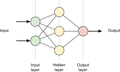
The magic of neural networks lies in fine-tuning the transformation of the input data as it’s pushed through the layers. This technique is known as back propagation and it is key to how neural networks appear to learn. The idea starts by feeding an input through the network and comparing the output with the expected result. The difference is passed through a cost function and then used to adjust the synapses a layer at a time from the output back to the input. Repeating this process with many different inputs results in the network starting to reflect the desired behaviour. The theory behind this is rather maths heavy; I’d recommend watching Neural Networks Demystified for an in-depth explanation.
To test my understanding I set about a writing a neural network that could learn the sine function. This would be a network that consisted of a single input neuron for x, three hidden neurons, and an output neuron that gave an approximation of sin(x). Both inputs and outputs are normalised to be between zero and one for simplicity. I trained it with a 100,000 iterations of only three inputs and then asked it to compute sin(x) for ten different inputs. Running the resultant code NeuralNetworkDemo shows how the network improves during training:
Learning...

Iteration | Cost
#       0 | 0.090582
#   10000 | 0.000709
#   20000 | 0.000343
#   30000 | 0.000225
#   40000 | 0.000167
#   50000 | 0.000132
#   60000 | 0.000109
#   70000 | 0.000093
#   80000 | 0.000081
#   90000 | 0.000072
#  100000 | 0.000065
Here we see that the value of the cost function, which quantifies the difference between the actual and expected outputs, diminishes every iteration. Once training has taken place we can then feed our ten different inputs into the network to compute the sine function:
------------ Paste into spreadsheet ------------
Input	Output			Target
0.0	0.9999873069902044	0.5
0.1	0.9998488493115462	0.7938926261462366
0.2	0.9983090528423926	0.9755282581475768
0.3	0.9833851545556364	0.9755282581475768
0.4	0.8745132768612006	0.7938926261462367
0.5	0.4985759605781311	0.5000000000000001
0.6	0.14886659877620845	0.2061073738537635
0.7	0.0367033795608045	0.024471741852423234
0.8	0.010115911146936	0.02447174185242318
0.9	0.0033188579267310124	0.20610737385376332
1.0	0.001293026219153508	0.4999999999999999
------------------------------------------------
As the output suggests, we can plot this as a graph:
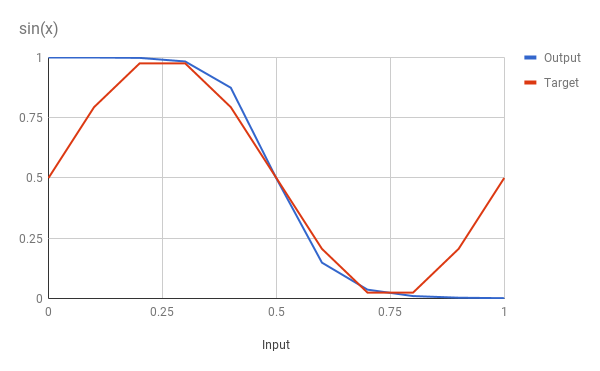
Given the limited set of training data we can see that the network has approximated the sine function quite well. The training data points 0.25, 0.5 and 0.75 are spot on, but the obvious discrepancies are at the extremities. It’s fair to say that these points cannot be inferred from the training data, but we may also be hitting a limitation of the number of neurons in the network, or the fact that the neurons do not support a bias.
Neuroevolution
Now that I had a basic understanding of genetic algorithms and neural networks I was finally ready to combine the two and delve into neuroevolution. What differentiates this technique from classic neural networks is that it does not require supervision to learn, rather it employs genetic algorithms to evolve the shape and values of the network.
In some respects this means that neuroevolution is simpler than regular neural networks since it doesn’t require backpropagation, which is often the most complex part of any implementation. Instead, the typical genetic algorithmic cycle of measuring fitness, genetic crossover and mutation iteratively trains a population of networks.
This conceptually simple idea quickly poses some difficult questions. How best to encode a neural network into genes and chromosomes? How can we mutate and combine networks to produce offspring? How can we allow beneficial traits in networks to evolve? The approach used by the Super Mario World demo is called NEAT, or NeuroEvolution of Augmenting Topologies.
Encoding
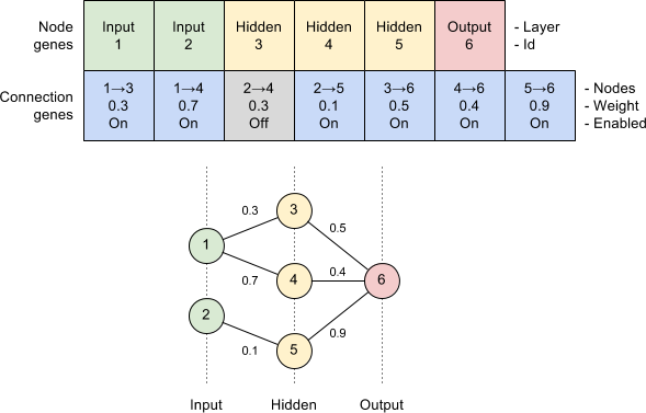
NEAT encodes neurons and synapses as node and connection genes respectively. A node gene simply states which layer it lives in, whereas a connection gene specifies which nodes it connects, its weight and an enabled flag. Additionally, every time a connection is created a global innovation number is incremented and assigned to the gene. We will see later how this innovation number is used to perform crossover.
Mutation
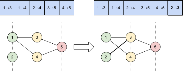
Mutation of the network can occur in several ways: connection weights are perturbed; unconnected nodes are connected; and connections are split by introducing new nodes. These basic transformations allow an arbitrarily complex neural network to evolve over time.
To illustrate, a connection gene mutation simply adds a new connection gene to join two previously unconnected nodes:
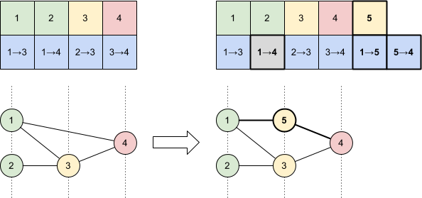
Whereas a node gene mutation disables an existing connection gene and adds a new node and connections in its place:
Crossover
Performing crossover of two networks with disparate topologies is seemingly a more complex problem. NEAT solves this by observing that connection genes with the same innovation number represent the same structural part of the network. This allows us to compute the difference between two networks by aligning their genes by innovation number.
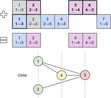
Genes that occur in both genomes are chosen randomly for the offspring, whereas those that are only present in one genome are inherited from the fittest parent. This simple algorithm allows breeding of neural networks without complex topological analysis.
For example, consider the following two parent networks:
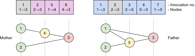
We can align their genes by innovation number and combine them as described to produce an offspring:
Species
An easily overlooked aspect is about how to protect innovation whilst ruthlessly pursuing survival of the fittest. The paper notes that early mutations often result in a decrease in the fitness of the network, meaning that they can be optimised out of existence before they have a chance to evolve into structures critical to long-term success.
NEAT tackles this problem by dividing the population up into species in order to restrict competition. Each species contains networks that have similar topology so that they compete against each other on a level playing field. Assigning an individual to a species involves computing a compatibility distance between itself and some arbitrary member; if that distance is within a given threshold then they also belong to that species. The compatibility distance is defined as a function of the number of disjoint genes between two genomes, so we can again use the innovation number to determine this as we saw with crossover.
Fitness
Finally, to evolve our network population we need to define a suitable fitness function that can measure success. The Super Mario World demo used a very simple concept for this – the number of pixels Mario had travelled to the right. For a platform game like Mario this makes sense, as the player typically starts on the left and moves right through the level to arrive at the finish. Other games will have different notions of success but it should always be relatively easy to define one.
Implementation
Unfortunately I didn’t get as far as I would have liked with implementing NEAT but you can see my work in progress under the neuroevolution package. A genetic model exists along with mutations and species categorisation; next steps would be crossover and fitness evaluation. Hopefully one day I’ll finish this and demonstrate a network evolving to play a simple video game.
In the meantime, for a complete implementation take a look at MarI/O which is the code behind the inspired Super Mario World demo.